Making Matplotlib plots

Preliminaries

This tutorial demonstrates the use of the Python version of Histogrammar. See the installation guide for installing version 1.0.4 or later.

It also uses the CMS public dataset. Use the following to create an iterator over the data (and refresh it if you use up all the events). You will need a network connection.

from histogrammar.tutorial import cmsdata
events = cmsdata.EventIterator()

Introduction

Histogrammar is an easy to use and powerful toolkit for aggregating data. It provides the building blocks and the back-end logic to make one or many dimensional histograms, bar charts, box plots, efficiency plots, etc. Before aggregating any data, the user declaratively writes the structure of the desired aggregation using Histogrammar’s simple and consistent grammar, and also provides the rules to fill the structure with data as a user defined function (usually a quick lambda function does the trick). Histogrammar takes care of the rest. The user does not write the logic that actually makes the histogram, no nested for loops, no map and reduce operations, no handling of bug-prone edge cases — this is taken care of by histogrammar’s implementation.

First histogram

Histogrammar’s scope and usage is best demonstrated with a series of examples. After covering the basics, a more interesting dataset will be used to motivate histogrammar’s more advanced features.

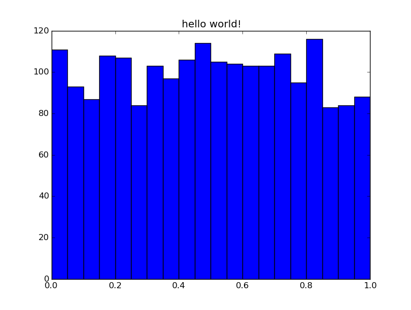
Lets make a histogram with 20 equally spaced bins of uniform random numbers, whose range is from zero to one. It makes one pass over a data stream. Let’s call this histogrammar’s “hello world!”:

import histogrammar as hg

# generate a stream of uniform random numbers
import random
data = [random.random() for i in range(2000)]

# aggregation structure and fill rule
histogram = hg.Bin(num=20, low=0, high=1, quantity=lambda x: x, value=hg.Count())

# fill the histogram!
for d in data:
    histogram.fill(d)

# quick plotting convenience method using matplotlib (if the user has this installed)
ax = histogram.plot.matplotlib(name="hello world!")

# to improve plot styling, try adding **kwargs suitable for plt.bar
#  e.g.: ax = histogram.plot.matplotlib(name="hello world!", color="slategrey", edgecolor="white")

If the plot doesn’t show up in your IPython terminal, you may need to turn interactive mode on, plt.ion(), or call plt.show() (after import matplotlib.pyplot as plt).

The first three arguments to hg.Bin are pretty self explanitory. num is the number of equal width bins to use. The low and high parameters are the lower and upper boundaries.

With hg.Bin, the user can also specify:

• underflow: what to do with data below the low edge;
• overflow: what to do with data above the high edge;
• nanflow: what to do with data that is not a number (NaN).

The default for these is Count().

Most of the action happens in value and quantity parameters.

Composability

quantity, the fill rule

quantity is the fill rule: a lambda or normal python function that is responsible for extracting the quantity we are interested in from a single data point in the dataset. Since our dataset in the above example was a list of numbers, not much happens in the fill rule. Often the data we are interested might be buried in a series of complicated objects. The quickest thing for an analyst to do in this case is usually loop over objects while extracting the elements of interest into an array. Then a second pass is made over the data to do the aggregation. The fill rule is where this logic belongs:

# The data of interest (value) is buried within some unweildy object (DataPoint)
class DataPoint(object):
    def __init__(self, value):
	    self.value = value

data = [DataPoint(random.random()) for i in xrange(2000)]
histogram = hg.Bin(num=20, low=0, high=1, quantity= lambda x: x.value, hg.Count())

What if we want to do something histogrammar doesn’t have built in, like making a histogram with a logarithmically spaced binning? One option is to take advantage of histogrammar’s use of user-defined fill rules.

import math
data = [random.random()*100000 for i in xrange(5000)]
histogram = hg.Bin(num=6, low=0, high=6, quantity=lambda x: math.log10(x), value=hg.Count())
for d in data:
    histogram.fill(d)

value, the aggregator

Finally, we give the value parameter a histogrammar object that is the actual aggregator. So far we have demonstrated Count. Count is a simple counter that adds one to a total each time it is called. At this point we can start to see histogrammar’s grammar taking shape. Notice that Bin is a noun, and Count is a verb. Count the number of data points that fall within each bin.

There are several primitives of this type available, such as Sum, Deviate, Minimize, Maximize, and more. They may not be so useful on their own, but the different aggregators each have their own fill method:

data = [random.random() for i in xrange(1000)]
counter = hg.Count()
minimum = hg.Minimize(lambda x: x)
deviate = hg.Deviate(lambda x: x)
for i, d in enumerate(data):
    counter.fill(d)
    minimum.fill(d)
    deviate.fill(d)
    # print aggregator state every 200th iteration
    if i % 200 == 0:
        print "\n - Iteration", i
        print counter
        print minimum
        print deviate

All the primitives except Count have a fill rule. To see why, we’ll generate a two dimensional dataset.

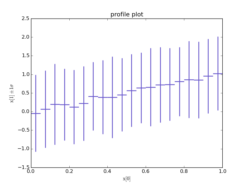
The x1 variables are normally distributed with a mean given by x2, which is a variable with a uniform distribution between 0 and 1. The variance of x1 is one.

x2 = [random.random() for i in range(5000)]
x1 = [random.gauss(x, 1) for x in x2]
data = zip(x1, x2)

h = hg.Bin(20, 0, 1, lambda x: x[1], hg.Deviate(lambda x: x[0]))
for d in data:
    h.fill(d)

ax = h.plot.matplotlib("profile plot", aspect=False, lw=2, color="slateblue")
ax.set_ylabel("$\\mathrm{x}[1] \\pm 1\\sigma$")
ax.set_xlabel("$\\mathrm{x}[0]$")

Note that a “profile plot” usually gives the error on the mean, and can be turned on by setting aspect=True.

Filling the histogram with data

As you have probably noticed, the histogram object is empty until filled with data. Part of what makes histogrammar powerful is the back-end implementation. Notice that the fill method of the [Bin][http://histogrammar.org/python/0.7/histogrammar.primitives.bin.Bin.html] object only has two arguments: datum (also the input to the fill rule) and an optional weight for that datum. How the aggregation is actually implemented under the hood is taken care of by histogrammar.

This includes the appropriate handling of nans, infs, and datapoints that fall above and below the high/low boundaries. For example:

data = [random.random() for i in range(2000)]

# add some "bad" values into the dataset
data.extend([float('nan'), float('inf'), float("-inf"), 100, -100])
h = hg.Bin(num=20, low=0, high=1, quantity=lambda x: x, value=hg.Count())
for d in data:
    h.fill(d)

# histogrammar has kept track of these
print "NaN counter:       ", histogram.nanflow
print "overflow counter:  ", histogram.overflow
print "underflow counter: ", histogram.underflow

The most efficient way to fill the initially empty aggregation depends on the computing environment of the user. On a single machine, a single pass over the data using the fill method is the best we can do. If, for example, we are working in a distributed computing cluster running [Apache Spark][http://spark.apache.org/] and our dataset was a large resilient distributed dataset (RDD) we would efficiently fill the aggregation like this (in a PySpark prompt) without using a for loop:

data.aggregate(histogram)(hg.increment, hg.combine)

increment is similar to fill, and hg.combine merges two aggregations into one. Notice what (h + h).plot.matplotlib() does.

Other pages in the documentation provide more detail on using histogrammar in different computing environments.

Exporting results

The aggregated data is easily accessible as attributes. If you are using an IPython terminal type h., or dir(h). Try printing `h.values`. If a plotting method doesn't exist for your histogrammar structure, this is how you extract the results.

Histogrammar also can export its results in a consistent [JSON][https://en.wikipedia.org/wiki/JSON] format. This allows results to be saved to disk in a standardized manner.

# as python objects (dicts, lists, etc.)
print h.toJson()

# and as a JSON string, ready to write to disk
import json
print json.dump(h.toJson())

Realistic Examples

The next series of examples follows the other tutorials and shows of some of the more advanced histogrammar aggregations and quick matplotlib plotting methods. First let’s load in the CMS data used in the other examples:

events = cmsdata.EventIterator()

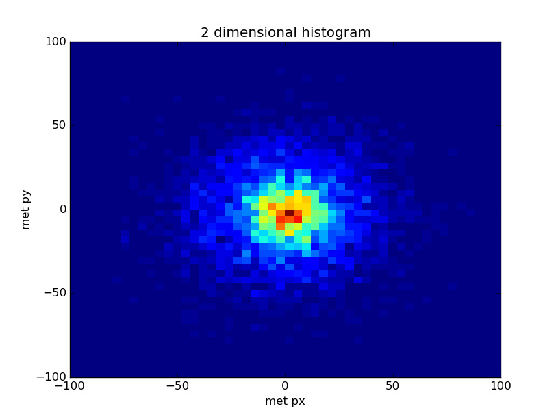
The following series of examples is meant to highlight histogrammars composability, and to highlight how this enables interesting aggregations to be easily made. As you may have noticed, from how Count can be used similarly to Bin, why not do a Bin of Bin of Count. This creates a 2 dimensional histogram:

hist2d = hg.Bin(50, -100, 100, lambda event: event.met.px,
             value = hg.Bin(50, -100, 100, lambda event: event.met.py))

for i, event in enumerate(events):
    if i == 5000: break
    hist2d.fill(event)

ax = hist2d.plot.matplotlib(name="2 dimensional histogram")
ax.set_ylabel("met py")
ax.set_xlabel("met px")